
▶ Intro
🎧 Spotify 팟캐스트 채널 <Linear Difressions>에서 '뭘 들어볼까~'하고 재밌는 에피소드를 찾던 중 발견! ✨

분석 데이터 기능들이 각양각색인 프로젝트를 관리하는 경우,
보통 각각의 기능들에 최적화된 여러 맞춤형 시스템들을 구축한다.
다만 이 과정에서 여러 문제들을 겪으며 Youtube는 완전히 다른 솔루션을 내놓는다.

바로, 아예 하나의 분석 데이터 시스템을 구축하기..!
요구사항과 조건들이 다른 기능들을 도대체 어떻게 하나의 시스템으로 통합할 수 있었는지, 하나로 통합하는 게 정말로 더 효율적인 방안인지 궁금해졌다.🤔
▶ Table of contents (목차)
- Summary
- Context (배경)
- Architecture
- Optimization Techniques
> Summary
There was increasing demand for data-driven applications at YouTube: reports and dashboards, embedded statistics in pages (no of views, likes,…), time-series monitoring, and ad-hoc analysis. Instead of building dedicated infrastructure for each use case, engineers at YouTube built a new SQL query engine — Procella. The engine is designed to address all of the four use cases. At the time of paper writing, Procella served hundreds of billions of daily queries on YouTube.
> Context
YouTube는 하루에 수조 개의 새로운 데이터 항목을 생성한다. 동영상 수, 수억 명의 크리에이터와 팬, 수십억 명 조회수, 시청 시간이 수십억 시간에 이르며, 이 데이터를 이용하는 기능이 총 4가지 존재한다.
| Definition | What it Requires | |
| Reporting and dashboarding | 콘텐츠 제작자와 YouTube 내부 이해관계자가 동영상과 채널의 실적을 이해하기 위한 실시간 대시보드 ex) How many views did the video earn right now? |
- Data volume is high - Low latency (tens of milliseconds) (requires real-time response time and access to fresh data) |
| Embedded statistics | 동영상의 좋아요나 조회수 등 다양한 실시간 통계 |
-Low latency (requires real-time updates since the values are constantly changing) |
| Monitoring | 보통 엔지니어가 내부적으로 사용 | - lower-query volume (since it is typically used internally by engineers) - but higher complexity |
| Ad-hoc analysis | 여러 YouTube 팀들(데이터 과학자, 비즈니스 분석가, 제품 관리자, 엔지니어)이 사용 ex)What's our number one video? How are the views compared to last year? |
- Data volume is low - Moderate latency (seconds to munites) - Querey patterns are unpredictable |
💡Low Latency: 낮은 지연시간
ex) 동영상의 좋아요/조회수 등의 통계는 유저 입장에서 최대한 fresh data(최신 데이터)를 알고 싶으니
latency(지연시간)이 최대한 낮아야 User Experience(UX)가 좋겠구나!
(Initially)
YouTube leveraged different technologies for data processing:Dremel for ad-hoc analytics, Bigtable for customer-facing dashboards, Monarchf for site health monitoring, and Vitess for embedded statistics.
(Pain Points)
However, using a dedicated tool for specific demands raises some challenges:
- There are too many ETL processes to load data to multiple systems.
💡ETL: 데이터를 추출(Extract)하고, 변환(Transform)하여 데이터 저장소에 로드(Load) 하는 일련의 프로세스 - Each system has a different interface, which increases learning code and reduces usability.
💡시스템들마다 다른 language와 API를 사용하기 때문에
➡ So you need to migrate data across these systems. - Some systems have performance and scalability issues when dealing with YouTube data.
(Solution)
To solve these pain points, YouTube built Procella, a new distributed query engine with a set of compelling features:
- Rich API: Procella supports a nearly complete implementation of standard SQL.
- High Scalability: Procella can achieve scalability more efficiently by separating storage and computing
- High Performance: Procella uses state-of-the-art query execution techniques with very low latency.
- Data Freshness: It supports high throughput and low latency data ingestion in batch and streaming.
💡Procella의 특징: Data Storage(데이터 스토리지)와 Computing(컴퓨팅)을 분리시켰다!
(참고)
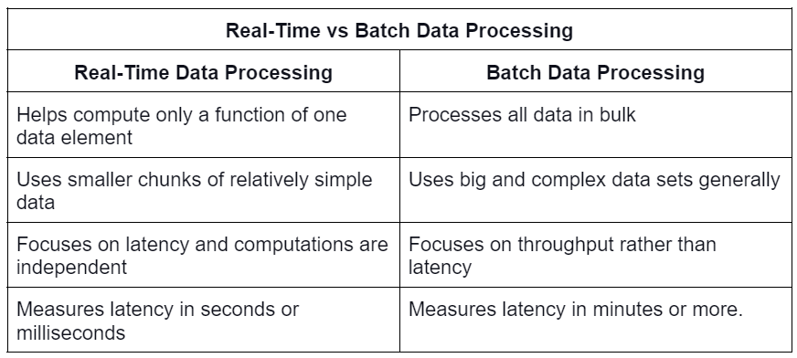
There are 2 different types of data
- Real-time data: streaming online data storage
- Batch data: off-line data storage
💡Latency(지연 시간) V.S. Response Time(응답 시간)
| Latency 지연 시간 | Response Time(응답 시간) |
| 요청이 처리되길 기다리는 시간으로, 서비스를 기다리며 latent(휴지) 상태인 시간을 말한다. |
클라이언트 관점에서 본 시간으로, 요청을 처리하는 실제 시간 외에도 네트워크 지연과 큐 지연도 포함한다. |
💡Throughput: 처리량
➡ 초당 처리 가능한 레코드수나 일정 크기의 데이터 집합으로 작업을 수행할 때 걸리는 전체 시간
💡Tail Latency (꼬리 지연 시간) = 상위 백분위 응답 시간
서비스의 사용자 경험에 직접 영향을 주기 때문에 중요하다.
e.g. Amazon 아마존은 내부 서비스의 respnose time 요구사항을 p999로 기술한다. p999는 요청 1000개 중 1개만 영향이 있음에도 말이다. 보통 response time이 가장 느린 요청을 경험한 고객들은 많은 구매를 해서 고객 중에서 계정에 가장 많은 데이터를 갖고 있어서다.
반면 p9999를 최적화하는 작업에는 비용이 너무 많이 들어 아마존이 추구하는 목표에 충분히 이익을 가져다주지 못한다고 여겨진다. 최상위 백분위는 통제할수 없는 임의 이벤트에 쉽게 영향을 받기 때문에 response time을 줄이기가 매우 어려워 이점은 더욱 줄어든다.
> Architecture
Procella is designed to run on Google infrastructure.
Google has one of the world’s most advanced distributed systems infrastructure.


The storage
All data is stored in Colossus, Google’s scalable file system. The storage has some differences when compared to the local disk:
- Data is immutable.
- Metadata operations such as listing files have higher latency than local file systems because they must communicate with Colossus’s metadata servers.
- All Colossus read or write operations can only be executed via RPC, which leads to higher cost and latency when there are many small operations.
The compute
All servers are run on Borg, Google’s cluster manager (imagine Kubernetes here, but Borg is the internal technology at Google). Running on Borg means there are some implications:
- Borg master can often tear down machines for maintenance and upgrades …
- A Borg cluster will have thousands of commodity machines with different hardware configurations, each with a different set of tasks with incomplete isolation. Thus, the task performance can be unpredictable. This implies that a system running on Borg must have fault-tolerance capability
💡일부로 maintenance 등을 위해 의도적으로 속도를 저하하기도 하는구나! (data throttling)
[The Data]
📁 Data Storage
As mentioned above, the data in Procella is stored separately in Colossus. Logically, Procella organizes into tables. Each table has multiple files, which are also referred to as tablets or partitions. The engine has its columnar format, Artus, but it also supports other formats, like Capacitor (the Dremel query engine format).
📁 Metadata Storage
Procella uses lightweight secondary structures such as (map of the location of the data) zone maps, bitmaps, bloom filters, partition, and sort keys. The metadata server provides this information for the root server during the query planning phase. These secondary structures are retrieved from the data file headers. Most metadata is stored in metadata stores such as BigTable.
📤 Table management
Table management is achieved by sending standard DDL commands (CREATE, ALTER, etc.) to the registration server (which will be covered in upcoming sections). The user can define information like column names, data types, partitioning, sorting information, etc. Users can specify expiration time or data compact configuration with the real-time tables.
💡 DDL 명령어(SQL): 데이터를 담는 그릇을 정의하는 언어
- CREATE: To add a new object to the database.
- ALTER: To change the structure of the database.
- DROP: To remove an existing object from the database.
- TRUNCATE: To remove all records from a table, including the space allocated to store this data.
⌛ Batch time ingestion

The typical approach for processing batch data for users in Procella is using offline batch processes (e.g., MapReduce) and then registering the data by making a DDL RPC to the register server.
During the data registration phase, the register server extracts the table-to-file mapping secondary structures from file headers. Moreover, Procella also leverages data servers (covered in the upcoming sections) to generate secondary structures if the required information is not in the file headers. The register servers are also responsible for sanity checks during the data registration phase. It validates schemas’s backward compatibility, prunes, and compacts schemas…
⌛ Real-time data ingestion
In Procella, the ingestion server is in charge of real-time data ingestion. Users can stream data into it using RPC or PubSub. When receiving the data, the ingestion server can apply some transform to align it with the table’s structure and append it to the write-ahead log in Colossus. They also send the data in parallel to the data server for real-time queries based on the data partitioning scheme. The data servers temporarily store data in the memory buffer for query processing.
Having the data flow in two parallel paths allows the data to be available to queries in near real-time while eventually being consistent with slower, durable ingestion. The queries can combine data from in-memory buffers and the on-disk tablets. Moreover, the querying-from-buffer can be turned off to ensure consistency with the trade-off of higher query latency.
💡 데이터 흐름이 two parallel paths(병렬)이면, 거의 실시간으로 쿼리(query)할 수 있구나!
💡 Buffer(버퍼): A와 B가 서로 입출력을 수행하는 데 생기는 속도차이를 극복하기 위해 사용하는 임시 저장 공간
e.g. Youtube 스트리밍: 서버로부터 동영상을 내려받은 부분(밝은 회색 ➡ 이게 버퍼!)

👏 Compaction
To make data more efficient for serving, the compaction server periodically compacts and repartitions the logs written by the ingestion servers into larger partitioned columnar files. The compaction server can apply user-defined SQL-based logic specified during table registration to reduce the data size by filtering, aggregating, or keeping only the latest value.
💡데이터의 규모가 대용량 되면서 ➡ 연산 시간을 크게 줄이고, 성능 향상을 위해
1) "Data Compression (데이터 압축)"
2) "Data Partitioning (데이터 분할)" = 큰 Table/Index를 작은 단위인 Partition으로 나눈다.
The Query Lifecycle
Let’s see how the internal query flows in Procella.

- Clients send the SQL queries to the Root Server (RS).
- The RS performs query rewrites, parsing, planning, and optimizations to generate the execution plan.
- The RS uses metadata such as partitioning and index information from the Metadata Server (MDS) to filter out unnecessary data files.
- The RS orchestrates the query execution through the different stages.
- The RS builds the query plan as a tree composed of query blocks as nodes and data streams as edges.
- The Data Servers (DS) are responsible for physical data processing. After receiving the execution plan from the RS or another DS, the DS executes the according query plan and sends the results back to the requestor (RS or DS)
- The plan starts with the lowest DS reading source data from Colosuss or the DS’s memory buffer. The query is carried out following the plan until it is finished.
- Once the RS receives the final results, it sends the response back to the client.
💡Data Shuffling의 목적: helps prevent bias during training, ensures randomness in batch selection, and prevents the model from learning patterns based on the order of the data.
> Optimization Techniques
💡Optimization(최적화): 주어진 문제에 대해 최소한의 비용으로 가장 최선의 목표를 찾는 과정
1. Caching
: (보다 빠르게 데이터에 접근하기 위해) 데이터나 값을 미리 복사해 놓는 임시 장소.
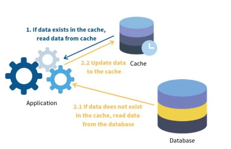
Procella employs multiple cache strategies to mitigate networking latency due to the separation of computing and storage:
- Colossus metadata caching: The file handles contain the mapping between the data blocks and the Colossus servers. Data Servers cache these handles to avoid too many file open calls to the Colossus.
- Header caching: The data servers cache the header information (e.g., column size and column’s min-max values) in the dedicated LRU cache.
- Data caching: The DS caches columnar data in a separate cache. The format Artus lets the data have the exact representation in memory and on disk, which makes it convenient to populate the cache.
- Metadata caching: To avoid bottlenecks due to remote calls to the metadata storage, the metadata servers cache the metadata in a local LRU cache.
- Affinity scheduling: Procella implements affinity scheduling to the data and metadata servers to ensure that the same data/metadata operations go to the same server. An important note is that the affinity is flexible; the request can be routed to a different server when the desired server is down. In this case, the cache hit is lower, but the query is guaranteed to be processed successfully. This property is important for high availability in Procella.
The caching strategies are designed so that when there is sufficient memory, Procella becomes an in-memory database.
2. Data format
The first version of Procella used the Capacitor data format, primarily aimed at large scans typical in analysis workloads. Since Procella is designed to cover several other use cases requiring fast lookups and range scans, YouTube decided to build a new format called Artus; let’s see some features of the format:
- It uses custom encoding to seek single rows without decompressing data efficiently. This makes the format more suitable for small-point lookups and range scans.
- Doing multi-pass adaptive encoding, e.g., first passes over the data to collect lightweight information (e.g., distinct values, min, max, etc.). It uses this information to determine the optimal encoding scheme. Besides that, Artus uses various methods to encode data, such as dictionary encoding, run-length, delta, etc.
- Artus chooses encodings that allow binary search for sorted columns, allowing fast lookups in O (logN) time.
- Instead of using representation for nested and repeated data types adopted by Capacitor and Parquet, Artus visualizes a table’s schema as a tree of fields and stores a separate column on disk for each field.
- Artus also implements many common filtering operations inside its API, which allows computation to be pushed down to the data format, leading to significant performance gain.
- Apart from the data schema, Artus also encodes encoding information, bloom filters, and min-max values to make many standard pruning operations possible without reading the actual data.
- Artus also supports inverted indexes.
3. Evaluation Engine
Many modern analytical use LLVM to compile the execution plan for native to achieve high evaluation performance. However, Procella needs to serve both analytical and high QPS demands, and for the latter, the compilation time can often affect the latency requirement. Thus, the Procella evaluation engine, Superluminal, takes a different approach:
- Using C++ template metaprogramming for code generation.
- Processing data in blocks to use vectorized computation and CPU cache-aware algorithms.
- Operating directly on encoding data.
- Processing structured data in an entirely columnar fashion.
- Pushing filters down the execution plan to the scan node allows the system only to scan the rows required for each column independently.
🤓 Fact: Superluminal powers the Google BigQuery BI and Google BigLake processing engines.
4. Partitioning and Indexing
Procella supports multi-level partitioning and clustering. Most fact tables are partitioned by date and clustered by multiple dimensions. Dimension tables would generally be partitioned and sorted by the dimension key. This enables Procella to prune tablets that do not need to be scanned and perform co-partitioned joins, avoiding moving data around.
The metadata server is responsible for storing and retrieving partition and index information. For high scalability, MDS is implemented as a distributed service. The in-memory structures are transformed from Bigtable (the metadata store) using various encoding schemes such as prefixes, delta, or run-length encoding. This ensures that Procella can deal with a vast amount of metadata in memory efficiently.
After filtering out the unwanted tablets, the data server uses bloom filters, min/max values, and other file-level metadata to minimize disk access based on the query filters. The data servers will cache this information on the LRU cache.
5. Distributed operations
(1) Distributed Joins
Procella has several join strategies that can be configured using hints or implicitly by the optimizer based on the layout and size of the data:
- Broadcast: One table side in the join operation is small enough to be loaded into the memory of each data server running the query.
- Co-partitioned: When fact and dimension tables are partitioned on the same join key, the data server only needs to load a small subset of the data to operate the join.
- Shuffle: When both tables of the join operations are large, data is shuffled on the join key to a set of intermediate servers.
- Pipelined: When the right side of the join is a complex query but has a high chance that it will result in a small data set, the right-size query will be executed first, and the result is sent to the servers in charge of the left-side query. In the end, this results in a broadcast-like join
- Remote lookup: In many cases, the dimension table is partitioned on the join key; however, the fact table is not. In such cases, the data server sends remote RPCs to the server in charge of dimension tablets to get the required keys and values for the joins.
(2) Addressing Tail Latency
Operating on commodity-shared hardware, individual machine failures are not rare. This makes achieving low tail latency difficult. Procella has some techniques to deal with this problem:
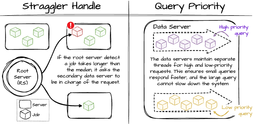
- The root server maintains data server response latency statistics while executing a query. If a request takes longer than the median, it asks the secondary data server to come and be in charge of the request. This can be achieved thanks to data being stored in Colossus, which makes the data available for every data server.
- The root server limits the requests to the data servers currently handling heavy queries to avoid putting more burden on these servers.
- The root server decorates the priority information for each request to the data servers. Generally, smaller queries will have higher priority, and larger ones will have lower priority. The data servers maintain separate threads for high and low-priority requests. This ensures small queries respond faster, and the large query cannot slow down other queries.
(3) Intermediate Merging
The final aggregation often becomes the bottleneck for queries with heavy aggregations as it needs to process large amounts of data in a single node. Thus, they add an intermediate operator right before the final aggregator, which acts as a data buffer. The operator can dynamically bring additional CPU threads to perform aggregations if the final aggregator cannot keep up the data in the buffer.
6. Query Optimization
(1) Virtual Tables
A common technique used to maximize the performance of low latency high QPS queries (needed for high volume reporting) is materialized views. The core idea is to generate multiple aggregates of the underlying base table and choose the right aggregate at query time (either manually or automatically).
Procella supports materialized views with some additional features to ensure optimal query performance:
- Index-aware aggregate selection: the materialized view in Procella chooses suitable tables based on physical data organization, such as clustering and partitioning.
- Stitched queries: the materialized view combines multiple tables to extract different metrics from each one using UNION ALL if they all have the dimensions in the query.
- Lambda architecture awareness: the materialized view combines multiple tables from batch and real-time flow using UNION ALL.
- Join awareness: the materialized view understands the joins and can automatically insert them in the query.
(3) Query Optimizer
Procella’s query optimizer uses static and adaptive query optimization techniques. During the query compilation phase, they use a rule-based optimizer. At query execution time, they use adaptive techniques (dynamically changing the plan properties such as the workers needed) to optimize physical operators based on statistics of the data used in the query.
Adaptive techniques simplify the Procella system, as they do not have to collect and maintain statistics on the data beforehand, especially when Procella is ingested at a very high rate. The adaptive techniques can be applied to aggregation, join, and sorting operations.
7. Serving Embedded Statistics
Procella powers various embedded statistical counters, such as views or likes, on high-traffic pages such as YouTube channel pages. The query for these use cases is straightforward: e.g., SELECT SUM(views) FROM Table WHERE video id = X, and the data volumes are relatively small.
However, each Procella instance needs to be able to serve over a million queries per second with millisecond latency for each query. Moreover, the user-facing statistical values are being rapidly updated (view increase, the user subscribes), so the query result must be updated in near real-time. Procella solves this problem by running these instances in “stats serving” mode:
-
When new data is registered, the registration server will notify the data servers so that they can load them into memory immediately.
-
Instead of operating as a separate instance, the metadata server’s functionality is compiled into the Root Server to reduce the RPC communication overheads between the root and metadata server.
-
The servers pre-load all metadata and asynchronously keep it updated to avoid remotely accessing metadata at query time, which incurs higher tail latencies.
-
Query plans are cached to eliminate parsing and planning overhead.
-
The root server batches requests for the same key and sends them to a single pair of primary and secondary data servers. This minimizes the number of RPCs required to serve simple queries.
-
The root and data server tasks are monitored so that Procella can move these tasks to other machines if there is a problem with the running machine.
-
Expensive optimizations and operations are turned off to avoid overheads.
▶ Outro
분석 데이터 기능들에 맞는 시스템들을 따로 구축하는 과정에서 ETL과정이 과도하게 많아지고, 시스템들마다 다른 인터페이스(언어, API 등)로 인한 비효율화 등의 문제들과 마주하게 된다는 사실을 알게 되었고,
각기 다른 인터페이스를 가진 시스템들을 통합하는 과정에서 최적화(Optimization)하기 위해 얼마나 많은 노력을 하는지 알 수 있었다.
✍새로 이해한 개념
- Latency / Tail Latency v.s. Response Time
- Throughput
- ETL process
- Data throttling
- DDL commands
- Buffer
- Data Compression / Data Partitioning
- Data Shuffling
- Optimization
📒영어사전
scalable 확장가능한
immutable 불변
append 추가하다
latency 지연시간
bring down 무너뜨리다
redundancy 중복성
periodically 주기적으로
prune 불필요한 가지를 치다
scalability 확장성
segregate 분리하다
출처
논문: <Procella: Unifying serving and analytical data at YouTube>
https://www.vldb.org/pvldb/vol12/p2022-chattopadhyay.pdf
Summary 글:
https://medium.com/thedeephub/procella-the-query-engine-at-youtube-e83b0c322e5e